CS2004 - Exam

• Run time: varies with the input and grows with input size (best case, worst case and average case).

  • $T(n)$: denotes the time an algorithm takes to execute, time versus input size $n$. It is measured by counting the number of primitive operations.

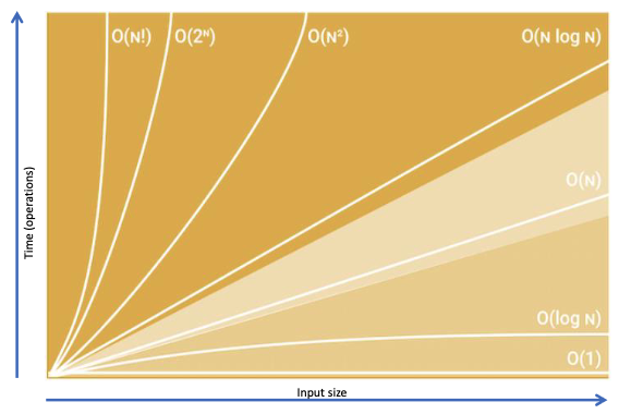
• Asymptotic Analysis: high-level description instead of implementation, analysis how time taken increases as input size increases. It determines the running time in Big-Oh notation.

  • To perform it:
    1. We find the worst-case number of primitive operations executed as a function of the input size, $T(n)$.
    2. We express this function with Big-Oh notation.

• Big-Oh Runtime Analysis:

  1. Find the input and what n represents.
  2. Calculate the primitive operations of the algorithm in terms of n.
  3. Drop the lower-order terms.
  4. Remove all constant factors.

• Polynomial time: when the number of steps is $O(n^k)$ where $k$ is not negative.

• Stacks are LIFO whereas queues are FIFO.

Counting Primitive Operations §

---

for i = 1 to n
    let a[i] = a[i] + x + y + 10
end for

• In line 1, we have n operations, however:

  • for i = 1 to n - 1 counts as n - 1 operations.
  • for i = 0 to n - 1 counts as n operations.

• In line 2, a counts as one operation and i counts as one. We have need to make sure to multiply it by the nesting value, in our case n.

Therefore, there are 9n operations in total.

---

Algorithm 5. ArrayMax(Arr)
Input: A 1-D numerical array Arr of size n>0
Let CurrentMax = a[0]
For i = 1 to n - 1
    If a[i] > CurrentMax Then CurrentMax = a[i]
End for
Output: CurrentMax, the largest value in Arr

• In line 3, we have 2 operations. We read $a_0$ and write to CurrentMax.

• In line 4, we have n - 1 operations.

• In line 5, we write to a and write to i, we read CurrentMax and check the comparison (>). We write to CurrentMax and read a and i again. So we have a total of 7(n - 1) operations.

The final total then is: $T(n)$ = $2+(n-1)+7(n-1)$ = $2+8n-8$ = $8n-6$ operations.

---

Algorithm 6. ArrayMax(Arr)
Input: A 2-D numerical array Arr of size n rows by m columns
Let CurrentMax = a[0][0]
For i = 0 to n - 1
    For j = 0 to m - 1
        If a[i][j] > CurrentMax Then CurrentMax = a[i][j]
    End For
End For
Output: CurrentMax, the largest value in Arr

• In line 3, we have 2 operations. We read a and CurrentMax.

• In line 4, we have n operations. This happens because for example, if n was equal to 5, the loop would iterate from i = 0 to i = 4, covering a total of 5 values for i: 0, 1, 2, 3 and 4 (5 operations).

• In line 6, we have m * n operations.

• In line 7, we have 9(m * n) operations.

Therefore, we have a total of: $T(n)$ = $2+n+(m\ast n)+9(m\ast n)$ = $10(m\ast n)+n+2$ operations.

Sorting and Searching §

---

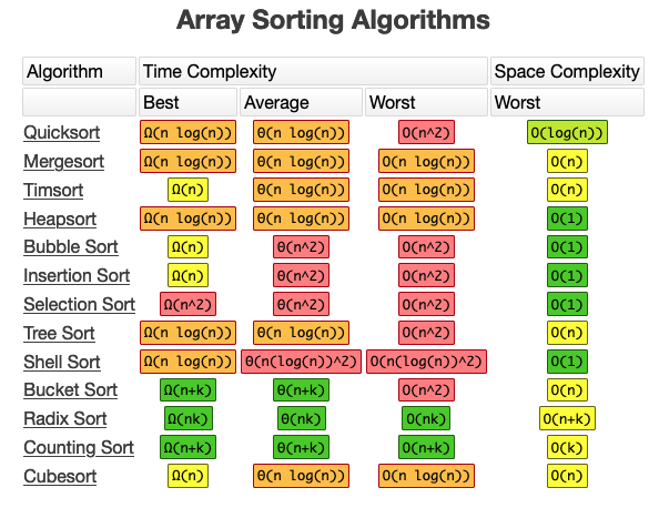
• Selection Sort ($O(n^2$): repeatedly finds the smallest element in the unsorted tail region of a list and moves it to the front.

We have:

• Sequential Search: every element is checked, linear search. List does not need to be sorted.
• Interval Search: binary search, divide and conquer. List must be sorted.

Binary search is a $O(lo{g}_2(n))$ algorithm, and linear search is $O(n)$. Therefore:

• Binary search is faster on sorted data.

Bubble Sort - O(n) §

---

Algorithm 1. BubbleSort(x)
Input: x - a list of n numbers
Let NoSwaps = False
While NoSwaps = False
    Let NoSwaps = True
    For i = 0 to n - 2
        If x[i] > x[i+1] then
            Swap x[i] and x[i+1]
            Let NoSwaps = False
        End If
    End For
End While
Output: x - sorted (ascending)

Worst-case: $O(n^2)$.

Quick Sort §

---

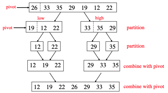
Algorithm 2. QuickSort(List, First, Last)
Input:
    List, the elements to be put into order
    First, the index of the first element
    Last, the index of the last element

If First < Last Then
    Let Pivot = PivotList(List, First, Last)
    Call QuickSort(List, First, Pivot-1)
    Call QuickSort(List, Pivot+1, Last)
End If
Output: List in a sorted order

Classes of Algorithms §

---

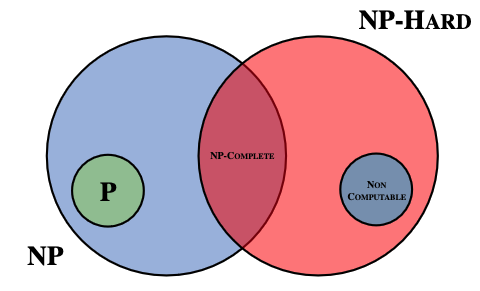
• P problems: solved in a reasonable amount of time (polynomial time), for example sorting.

• NP problems: difficult to solve in a reasonable amount of time but easy to verify the solution, problems involving decision making (non-deterministic).

  • NP-hard problems: very very difficult, difficult to verify in polynomial time.
  • NP-complete problems: hardest problems, verifiable in polynomial time but the complexities are greater. No polynomial-time algorithm is discovered for any NP-complete problems. Examples are: the travelling salesperson problem and finding the shortest common superstring.

• If a polynomial time algorithm is found for any problem in NP-complete, then every problem in NP can be solved in polynomial time.

Hill Climbing Algorithm §

---

Algorithm 1. RMHC(ITER)  
Input: ITER- the number of iterations to run for  
1) Let S be a random point in the search space,  
let F be its fitness  
2) For i = 1 to ITER (number of iterations)  
3)   Let S’ be a random point close to S,  
     Let F’ be its fitness  
4)   If F’ is better than F Then  
5)     Let S = S’ and Let F = F’  
6)   End If  
7) End For  
Output: S- a solution

1. Initialize the current solution as a random binary string.
2. Evaluate the fitness of the current solution using the fitness function.
3. Repeat until a stopping condition is met:
     a. Generate all neighbors of the current solution by flipping a single bit.
     b. Evaluate the fitness of each neighbor.
     c. Select the neighbor with the best fitness value.
     d. If the best neighbor has a better fitness than the current solution, set it as the new current solution.
     e. Otherwise, stop and return the current solution as the best solution found.

Holland’s GA Algorithm §

---

Input: The GA parameters: NG, PS, CP, MP and n  
The Fitness Function  
1) Generate PS random Chromosomes of length n  
2) For i = 1 to NG  
3)   Crossover Population, with chance CP per Chromosome  
4)   Mutate all the Population, with chance MP per gene  
5)   Kill off (or fix) all Invalid Chromosomes  
6)   Survival of Fittest, e.g. Roulette Wheel  
7) End For  
Output: The best solution to the problem is the Chromosome  
in the last generation (the NGth population) which  
has the best fitness value

Evolutionary Programming §

---

Input: Population size, number of generations  
and Fitness Function  
1) Create the initial population  
2) For i = 1 to number of generations  
3)  Mutate the population  
4)  Apply Tournament Selection  
5) End For  
Output: Return the best individual

• An algorithm is a step-by-step procedure or set of rules used to solve a specific problem or accomplish a particular task. It is a well-defined and unambiguous sequence of instructions designed to solve a problem in a finite amount of time.

• Big-T, also known as Theta notation (Θ), is a mathematical notation used in computer science to describe the asymptotic behaviour or growth rate of an algorithm’s time complexity. It represents the tight bound or upper and lower limits of the running time of an algorithm as the input size approaches infinity. In other words, Big-T provides a range of functions that bound the algorithm’s performance.

• Big-O notation (O) is another mathematical notation used in computer science to describe the upper bound or worst-case behaviour of an algorithm’s time complexity. It provides a way to characterise the maximum amount of resources (usually time or space) that an algorithm requires to solve a problem. In other words, Big-O notation represents an algorithm’s upper limit efficiency.

• Bubble sort is a simple sorting algorithm that works by repeatedly swapping adjacent elements if they are in the wrong order. The algorithm gets its name from the way smaller elements “bubble” to the top of the list during each pass.

• Quick sort is a divide-and-conquer algorithm that works by selecting a pivot element from the array and partitioning the other elements into two sub-arrays, according to whether they are less than or greater than the pivot. The sub-arrays are then recursively sorted.

• Radix sort is a non-comparative sorting algorithm that sorts elements based on their digits or characters. It works by processing the digits or characters of the elements from the least significant digit to the most significant digit (or vice versa).

• NP-Complete problems are a class of challenging computational problems that lack efficient polynomial-time algorithms. To solve them, approximation algorithms and heuristics are typically employed to find near-optimal solutions within reasonable time limits. One example of an NP-Complete problem is the Traveling Salesman Problem (TSP). The TSP asks for the shortest possible route that a salesman can take to visit a given set of cities exactly once and return to the starting city. The problem’s difficulty lies in the exponential growth of possible routes as the number of cities increases.

• Primitive operators are fundamental building blocks that perform elementary operations, such as arithmetic calculations, logical operations, or basic data manipulations. They are usually highly optimised and execute efficiently due to their direct implementation in the language or hardware.

• Data clustering is a technique used in unsupervised machine learning to group similar data points together based on their characteristics or attributes. The goal is to identify patterns, similarities, or relationships within a dataset without prior knowledge of the classes or labels. Bin Packing problem is a combinatorial optimisation problem that deals with efficiently packing a set of items into a fixed number of bins or containers. The objective is to minimise the number of bins used while ensuring that the total size or weight of items does not exceed the bin’s capacity. In summary, data clustering is a technique for grouping similar data points together based on their characteristics, while the Bin Packing problem is an optimisation problem concerned with packing items into bins to minimise the number of bins used.

• Evolutionary Programming (EP) and Genetic Algorithms (GA) are both evolutionary computation techniques inspired by natural evolution, but they differ in their approach to problem-solving and the way they handle population dynamics. EP focuses on optimising individual solutions using real-valued representations, employs self-adaptation, and is suitable for continuous optimisation. On the other hand, GA focuses on evolving populations of solutions using binary representations, employs fixed population size, and can handle a wider range of problem types, including both discrete and continuous optimisation.

• A heuristic is a technique or rule of thumb used to guide the search process towards more promising or favourable paths. Heuristics provide a practical way to make informed decisions based on available information and reduce the search space, thereby improving the efficiency of search algorithms.

• The key difference between P and NP classes is that P represents problems that can be efficiently solved, while NP represents problems for which solutions can be efficiently verified but may not be efficiently found.

Similarities and Differences: Random Mutation Hill Climbing (RMHC), Random Restart Hill Climbing, and Simulated Annealing are all stochastic search algorithms used for optimisation problems. Here are the similarities and differences between these algorithms:

Similarities:

• They all belong to the general class of local search algorithms.
• They iteratively explore the search space to find better solutions.
• They can get trapped in local optima if not properly guided.

Differences:

• RMHC focuses on making random mutations to the current solution and accepts the new solution if it is better. It doesn’t consider the direction of improvement or probability distributions.

• Random Restart Hill Climbing periodically restarts the search from a random initial solution to escape local optima. It performs multiple independent runs and keeps the best solution found across all restarts.

• Simulated Annealing uses a probabilistic approach to accept worse solutions in the early stages of the search. It gradually reduces the acceptance of worse solutions over time, mimicking the annealing process in metallurgy.

• The ”No Free Lunch” (NFL) theorem for heuristic search techniques is a fundamental result in the field of optimisation and machine learning. It states that, on average, no one heuristic search algorithm is universally better than all others across all possible problems.

---

5.5) The Ant Colony Optimization (ACO) algorithm is a metaheuristic approach inspired by the foraging behavior of ants. It is commonly used to solve combinatorial optimization problems such as the Traveling Salesman Problem (TSP).

• Route Selection: In the ACO algorithm, artificial ants are used to explore the solution space. Each ant builds a solution by iteratively selecting the next city to visit based on certain criteria, such as the amount of pheromone deposited on the edges and the heuristic information. The ants probabilistically choose their next city, with higher probabilities given to cities with higher pheromone levels or shorter distances.

• Pheromone Update: After each ant completes its tour, the pheromone levels on the edges are updated. The amount of pheromone deposited on an edge is typically proportional to the quality of the corresponding solution. Ants that find better solutions deposit more pheromone, while ants that find suboptimal solutions deposit less. This update of pheromone trails represents the collective learning of the ant colony and guides the search towards promising regions of the solution space.

• Pheromone Evaporation: Pheromone trails have a tendency to evaporate over time in the ACO algorithm. This is done to avoid the convergence of the search to suboptimal solutions and promote exploration of new paths. Pheromone evaporation ensures that the influence of outdated or less desirable solutions diminishes over iterations, allowing the ants to focus on better paths.

The combination of route selection, pheromone update, and pheromone evaporation in ACO contributes to an iterative process where the ants explore the search space, deposit pheromone based on the quality of solutions, and gradually converge towards better solutions. The positive feedback mechanism of pheromone reinforcement and the exploration-exploitation balance achieved through pheromone evaporation allow the algorithm to effectively search for high-quality solutions in complex optimization problems like the TSP.

5.6) Swarm Intelligence (SI) is a field that studies the collective behavior of natural and artificial systems composed of many individuals. Two properties of swarm intelligence are:

• Emergence: Swarm intelligence exhibits emergent behavior, which means that complex global patterns or behavior arise from the interactions and local behaviors of individual entities within the swarm. The collective behavior of the swarm is not explicitly designed or controlled by a central authority but emerges from the interactions and local rules followed by the individuals. In the case of ACO, emergent behavior is observed as the colony of artificial ants collectively finds good solutions to the TSP.

• Self-Organization: Swarm intelligence systems exhibit self-organization, which refers to the ability of individuals within the swarm to organize themselves without external coordination or central control. Each individual in the swarm follows simple rules and interacts with its neighbors or environment, leading to self-organized patterns or solutions that adapt to changing conditions. In ACO, the ants self-organize their exploration and exploitation of the solution space through the use of pheromone trails and local heuristics, resulting in the emergence of effective solutions to the TSP.