Heuristic Seach, Hill Climbing and Simulated Annealing

Heuristic Search §

---

Some difficult problems (NP-hard) cannot be solved in a straightforward manner.

We need to develop approximation algorithms to solve these problems.

Heuristic Search can be used to try and find a solution.

We search for the best solution from a very large number of potential solutions.

However, it might not always find the best solution.

We score the worth of each solution using a Fitness Function.

We try to find a solution that minimises and maximises the fitness, depending on how we rate the solution.

The computational complexity of Heuristic search methods is often very difficult to define.

We therefore often rate their performance in terms of the number of fitness function calls.

• We compute the Big O of this function.

We aim to choose the method that finds us the global optimum in the smallest number of fitness function evaluations.

No Free Lunch §

---

This theorem states that just because method X is great at solving problem Y it might be no use at solving problem Z.

• Even if problem Y and Z are very, very similar.

Random Mutation Hill Climbing (RMHC) §

---

Aims to find a point in the search space that maximises some objective function (fitness).

The RMHC algorithm starts off at some random point in the search space.

It then looks randomly at its close neighbours until it finds one with a better fitness.

The hill climbing algorithm then continues searching for improvement from this new point.

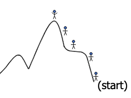
This is rather like the analogy of a hill walker trying to climb up a hill in the fog. They feel around themselves until they find a nearby direction that goes up. They then move to this higher point and continue searching.

Algorithm 1. RMHC(ITER)  
Input: ITER- the number of iterations to run for  
1) Let S be a random point in the search space,  
    let F be its fitness  
2) For i = 1 to ITER (number of iterations)  
3)   Let S’ be a random point close to S,  
     Let F’ be its fitness  
4)   If F’ is better than F Then  
5)     Let S = S’ and Let F = F’  
6)   End If  
7) End For  
Output: S- a solution

It can easily get “stuck” in a local optima:

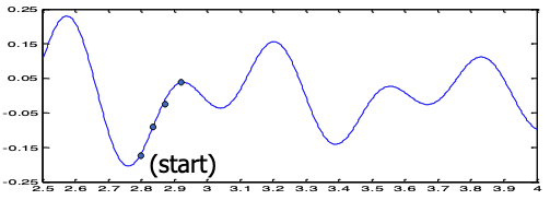
From the starting point, the algorithm will never reach the global optima.

Random Start §

---

For $n$ weights, we wanting to randomly create a starting arrangement, any will do.

We will simulate n tosses of a coin and put each weight on the left or right hand side of the scales

If we have a random integer $x\ge 0$ then what do we get if we modulo it by 2?

• If $x$ is even we get 0.
• If $x$ is odd we get 1.
• Hence we generate a random integer $x\ge 0$ and then set each $s_i$ to $x$
  modulo 2 (a new $x$ for each $s_i$).

Algorithm 2. RandomStart(n)  
Input: n- the number of weights  
1) Let S be a n length binary string  
    (or array)  
2) For i = 1 to n  
3)   Let si = |Random Integer| Mod 2  
4) End For  
Output: S- a random solution to the Scales Problem

Random Small Change §

---

We need a small change that creates $Sʹ$ from $S$ such that $S$ and $Sʹ$ are close.

• The change must be the smallest we can do…

We could do this by choosing a random weight and reversing the side that it is on.

Thus we generate a random $i$ and then look to see what value $s_i$ is:

• If $s_i$ = 0 then we set $s_i$ = 1
• If $s_i$ = 1 then we set $s_i$ = 0

Algorithm 3. SmallChange(Sold)  
Input: S_old - A binary string of length n
1) Let S = S_old
2) Let i be a random integer between 1 and n inclusive  
3) If si = 0 Then
4)   Let si = 1
5) Else  
6)   Let si = 0  
Output: S - a solution to the Scales Problem close to S_old

Test Scales Problem §

---

We test our RMHC algorithm on the first 1000 primes numbers.

We will run the algorithm for 1000 iterations and see how well it does.

• The choice for the number of iterations is “arbitrary”.

Convergence Graphs §

---

For ten runs:

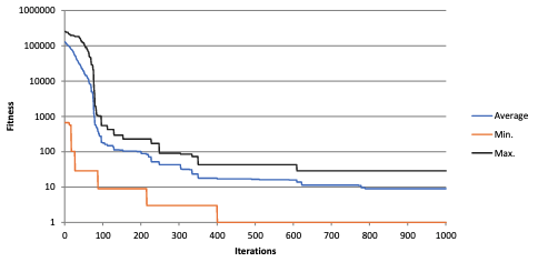
High variability of results, due to being trapped in local optima.

An average best fitness of 9.0.

Stochastic Hill Climbing §

---

The RMHC algorithm can have very variable performance.

We need to improve upon it to escape local optima.

We can do this by letting the algorithm accept worse fitness function values during its search.

This is the basic of the Stochastic Hill Climbing (SHC) algorithm:

• The change of accepting is a function of how bad the change is.
• A very bad change will have a small chance of being accepted.
• A slightly bad change will be accepted more often.
• Many ways of doing this, for example relies on decision function.

We accept (line 4 in the RMHC algorithm) a new solution according to the following equation:

$Pr(accept)$ = $\frac{1}{1+e^{(}{f}^{\prime }-f)/T}$

Here:

• $f^{\prime }$ is the new fitness (line 3 in the RMHC algorithm).
• $f$ is the old fitness.
• $T$ is a parameter (set to 25 for the 1000 primes scales problem).

The correct choice of $T$ can be very difficult.

Note that $f^{\prime }$ and $f$ should be “swapped” (order) for maximisation problem.

We get an average best of 8.0.

Random Restart Hill Climbing §

---

Very effective version of the Hill Climbing algorithm is the Random Restart (RRHC) version.

Here we run the normal RMHC algorithm a number of times and record the best.

• For example, we start off in different sections of the search space.
• For example, we might run it 10 times for 100 iterations rather than once for 1000 iterations.

For our Scales example we get an average best of 6.2.

Simulated Annealing §

---

It is another attempt to improve the Hill Climbing algorithm.

It allows a worse solution to be accepted so that local maximums can be circumnavigated.

• Sometimes you need to search and explore instead of always improve.

The term “annealing” refers to the fact that the chances of accepting a worse solution reduces as the algorithm progresses.

• An analogy to the annealing process in metallurgy.
• When you take a molten hot metal and you cool it down slowly for it to reach its stable form.

The annealing process is simulated through maintaining a slow decreasing temperature.

This temperature should reach zero at the end of the algorithm’s run.

• If temperature is very high: the algorithm is more likely to accept worst solutions.
• If temperature is zero: the algorithm behaves like HC - accepts better solutions.

Note that the parameters $T_0$ (starting temperature) and $\lambda$ (cooling rate) need defining, along with the acceptance function PR.

Note that if ITER is known, then we can calculate a value for $\lambda$.

For $T_{ITER}$ we choose a small value greater than zero, for example 0.001.

• $T_{i+1}$ = $\lambda T_i$
• $T_1$ = $\lambda T_0$
• $T_2$ = $\lambda T_1$ = $\lambda \lambda T_0$ = ${\lambda }^2{T}_0$
• $T_3$ = $\lambda T_2$ = $\lambda \lambda T_1$ = $\lambda \lambda \lambda T_0$ = ${\lambda }^3{T}_0$
• $Ti+1$ = ${\lambda }^{i+1}{T}_0$
• $T_{ITER}$ = ${\lambda }^{ITER}{T}_0$
• ${\lambda }^{ITER}$ = $\frac{T_{ITER}}{T_0}$
• $\lambda$ = $\sqrt[ITER]{\frac{T_{ITER}}{T_0}}$

So now we only have two parameters to determine, $T_0$ and $ITER$.

$ITER$ can be selected by trial and error, the algorithm is very fast so we can select a large value and reduce it if necessary. For example, 1000 in our 1000 Primes Scales example.

Determining $T_0$ can be a problem:

• Too small and the algorithm will behave like a hill climber.
• Too large and the algorithm may never converge.

The acceptance function PR is defined as follows:

$PR(f^{\prime },f,T_i)$ = $exp\frac{-\Delta f}{T_i}$

where $\Delta f$ = $|f^{\prime }-f|$

Note that $|x|$ means the absolute value of $x$, and equals $-x$ if $x<0$ or $x$ if $x\ge 0$.

• Loss (or change) is how much worse a neighbouring state is compared to the current state.
• If $|f^{\prime }-f|$ is close to zero PR will be 1, therefore we’ll accept the new solution.
• If $|f^{\prime }-f|$ is large, the new solution is worse than our old solution.
  • If $T$ is small, it is very unlikely we’ll accept the new solution (PR - will be very small).
  • If $T$ is large, it is likely that we’ll accept the solution even the new solution is worse.

Results Summary §

---

The methods performed as follows:

• RMHC: 9.0
• SHC: 8.0
• RRHC: 6.2
• SA: 5.8

However, these results were only from 10 runs for 1000 iteration.

They should have been run for maybe 100 repeats of perhaps 10000 iterations?

Maybe real numbers instead of prime numbers?

About HC and SA §

---

All of HC and the SA algorithms search for a good solution by starting at a random point and then examining neighbouring points.

This type of search is known as a local or neighbourhood search methods.